Time Series Analysis: Arrival Times of NYC Essential Agencies.
Distinct ARIMA models were used to analyze and predict the response times for incidents involving the NYPD and the FDNY from 2015 through 2019.
Keywords: ARIMA; autoarima; NYPD; FDNY; time series; forecasts

Intro
This dataset was provided by the Mayor’s Office of Operations (OPS) and can be found on NYC Open data. OPS tracks and reports the 911 calls civilians make and the time, measured in seconds, it takes for each call to reach the appropriate responding agency. This dataset provides multiple attributes such as “week start date”, “call to first pickup”, “call to FDNY pickup”, “call to NYPD pickup”, etc….
The need to track the performance of these agencies is important from a civilian perspective. Residents would like to know how well the NYPD can arrive to a critical incident, such as a shooting. Residents can hold these agencies accountable, but this also seems vital to the internal staff of every agency. To avoid any public scrutiny from a lack of performance, I am certain NYPD or FDNY upper management tracks how well their team can handle high pressure situations. A way to evaluate their team is to see how well they can arrive to a scene and provide their essential service.
The attribute this article will focus on is “call to agency arrival.” This is a metric that provides the average time, in seconds, it took per week for the agency to arrive at a scene. More specifically, this metric begins at the very moment the call enters the 911 system, to when an agency arrives on-scene. Other attributes, such as “call to agency dispatch” and “call to agency job creation” could have been evaluated. However, missing values did not make the time series easy to interpret.
Methods
ARIMA model
The individual time series will be evaluated using the auto.arima function from R. The assumptions that each time series are both auto regressive (AR) and moving average (MA) are dealt by the function.

In general, we say that 𝑌𝑡 from the equation above is a mixed autoregressive moving average process. Where p specifies the order of the AR process and q specifies the order of the MA process. There are additional parameters that can be passed through the auto.arima function, one of which specifies how many times R will difference the time series.
NYPD
The NYPD respond to incidents under the categories of “Critical”, “Serious”, and “Non-Critical.” Critical incidents include “Shots fired, assist police officer, robbery, burglary, larceny from person, assault w/ knife, assault w/ weapon, unusual incident.” While serious incidents fall under, “Auto theft, other larceny, other assault, roving band.”

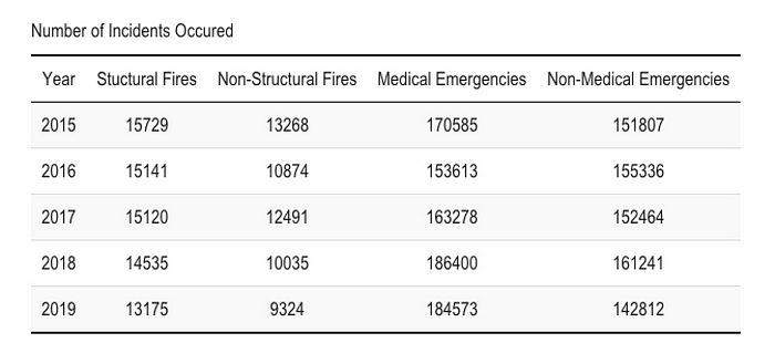
Table 1 provides a summary of the number of incidents NYPD personnel respond to every year. With the NYPD responding to serious incidents the most every year.

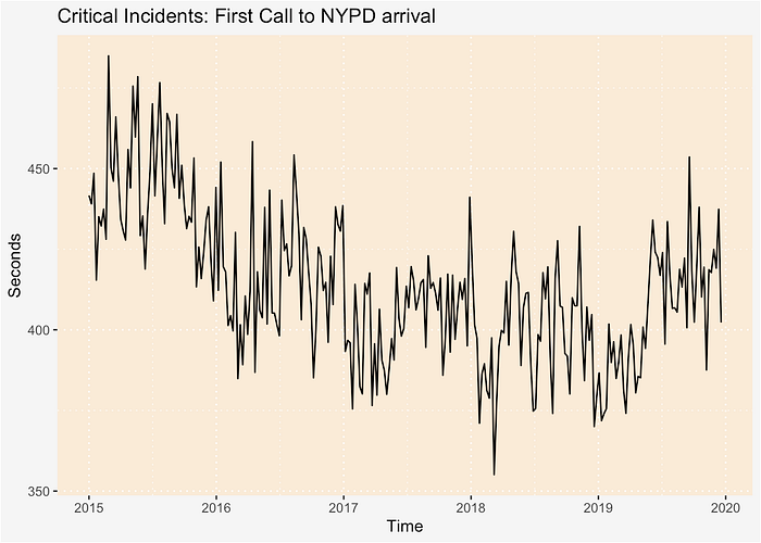
The first plot from figure 1 displays the three-time series, each for the types of incidents the NYPD respond to. We see that the NYPD arrive to critical incidents the quickest. A further look at the critical incidents time series reveals a decreasing trend in NYPD arrival time to incidents until the middle of 2017. Then fluctuations appear until the end of 2019.
For the purpose of the article, we will focus our attention in forecasting the critical incidents time series. We can assume these time series are non-stationary, this leads us to exploring what the differenced time series will look like. When differencing the data, we take the arrival time from week 1 of 2015 and subtract this time from the arrival time of week 2. This is done sequentially, for the following weeks leading up to the end of 2019. A plot of the differenced NYPD time series is shown below.
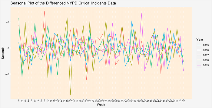
From figure 2, fluctuations appear to exist in the differenced time series. However, most of the time series is bounded between -40 and 40 seconds. We assume this data is stationary and can forecast the call to NYPD arrival time for critical incidents.
FDNY
The New York Fire Department respond to “Structural Fires”, “Non-Structural Fires”, “Medical Emergencies” and “Non-Medical Emergencies.” Structural fires include FDNY personnel responding to fires in “commercial, residential, public and vacant buildings.”
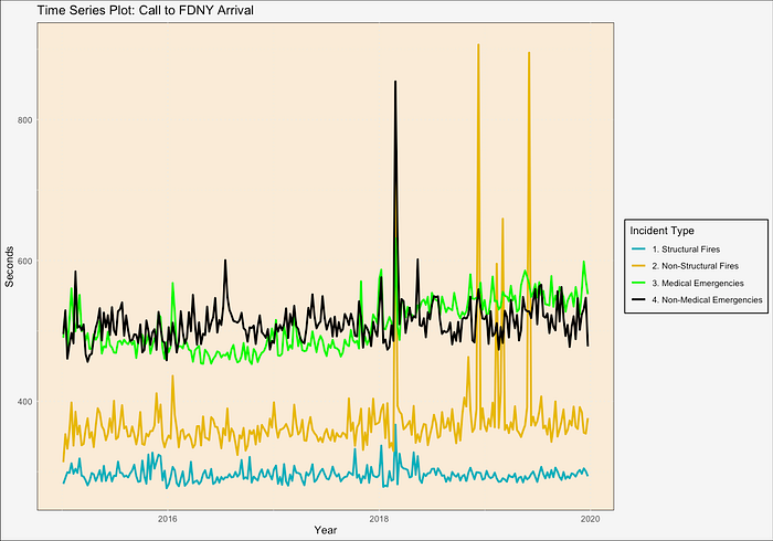
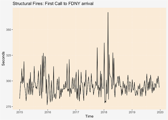
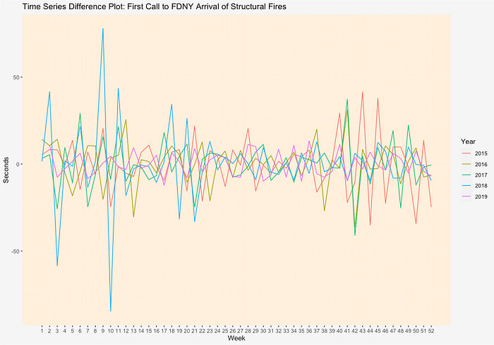
The first plot in figure 3 shows us that FDNY personnel arrive to structural fire incidents the quickest, when compared to the other three incidents. There appears to be a strange spike in response times for all incident types. The data dictionary advises that if the volume of the incident surpasses a point, response times will degenerate. For the purpose of this article, we will focus on forecasting incidents involving structural fires. The second plot from figure 3 displays fluctuations in the structural fires time series.
ARIMA modeling of NYPD data
We fit an ARIMA model, using the differenced first call to agency arrival times of the NYPD. We are returned an ARIMA(0,1,3). A model summary is found below.
Three moving-average parameters are used, along with a constant auto-regressive parameter.
From figure 5, the plot on the top displays a time series plot of the residuals from our model. For most of the time series, the residuals are bounded between -25 and 25 seconds. An auto-correlation plot is displayed, as well as a density plot that shows the residuals approximate a normal distribution. Lags 1 through 5 shows little to no autocorrelation.
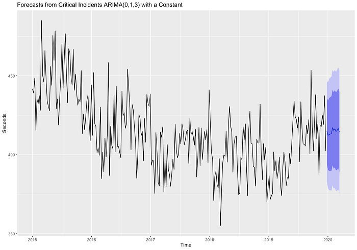
The Ljung-Box test was used to evaluate if this model is significant. We are given a test statistic, Q* = 47.74, with the residuals having 48 degrees of freedom. We compare this statistic to Q, the value of the upper tail chi-squared test, evaluated at an alpha level = 0.05 with 48 degrees of freedom. Q = 65.17. We see that Q* < Q, thus we fail to reject our null hypothesis: This ARIMA(0,1,3) model does not exhibit lack of fit. We conclude our null hypothesis. The bottom plot of figure 5 produces a 12-week forecast of the critical incidents time series. The dark blue region represents a 95% confidence interval, while the light blue shaded region represents an 80% confidence interval.
ARIMA modeling of FDNY data
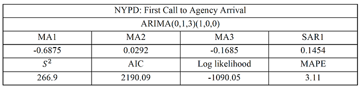
Using the differenced structural fires time series, we fit an ARIMA model and are returned these coefficients.
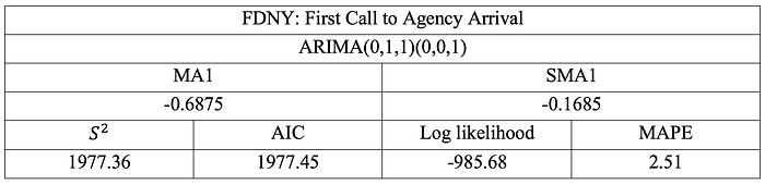
We estimate that an MA(1) with a constant, using the differenced time series, forecasts the call to FDNY arrival time the best. This AIC value is lower compared to the NYPD ARIMA model. This low AIC value can be attributed to the fact that we only use one moving-average parameter, and one moving-average constant.
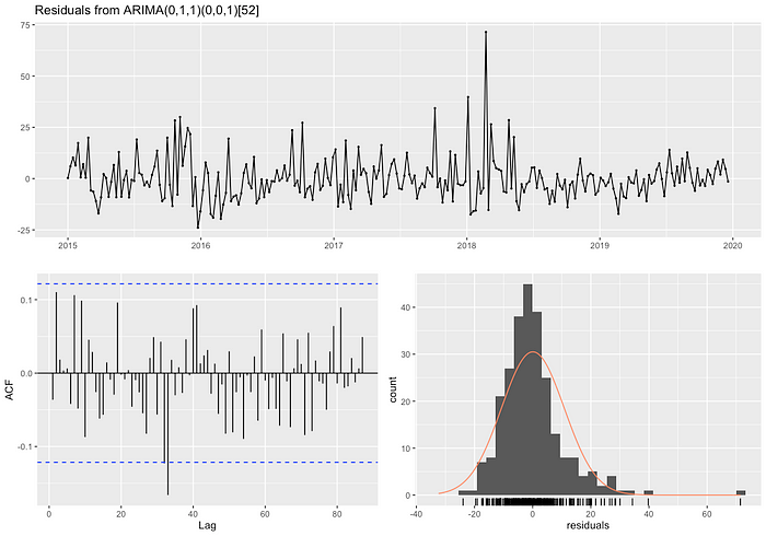

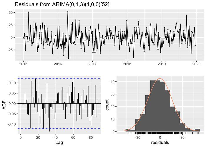
We can see a time series plot of the residuals from the ARIMA(0,1,1) model on the top. Most of the residuals are bounded between 25 and -25 seconds, with few fluctuations existing. The first five lags of the ACF plot are bounded by dashed blue lines. The lines represent that the values are bounded in the 95% confidence interval. The values in the plot show that lagged residuals have little to no autocorrelation.
The Ljung-Box test is used again to evaluate the lack of fit of this model. We state the null hypothesis, this ARIMA(0,1,1) model does not exhibit lack of fit. The test statistic is Q* = 50.33, with the residuals having 50 degrees of freedom. We compare this statistic to Q, the value of the upper tail chi-squared test, evaluated at an alpha level = 0.05 with 50 degrees of freedom. Q = 67.50. We see that Q* < Q. We fail to reject the null hypothesis, and conclude that this ARIMA(0,1,1) model does not exhibit lack of fit.
The forecast plot from figure 6 displays the estimated call to FDNY arrival times for 2020. We see that there are minimal fluctuations throughout the forecasted year. The estimated values eventually stabilize in 2021.
Conclusion
One forecasting technique for distinct NYC 911 end-to-end data has been presented. The ARIMA forecasting model can be applied once the time series being studied is seen as stationary. We forecasted our time series data, after the data has been differenced. As seen from the time observations from 2015, through the end of 2019, the arrival times for both city agencies are not linear. Attempting a non-linear forecasting technique can be done to work with the reported arrival times.
We can assess how accurate our forecasts are, by comparing our estimated values, to the arrival times of the agencies during the first eight weeks of 2020.
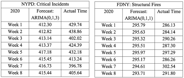
The forecast and the actual arrival times are measured in seconds. Looking at week 1 of table 7, the ARIMA(0,1,3) forecasted that on average, NYPD personnel will arrive to an incident from when a 911 call is initiated, in 412.30 seconds. We compared that to the actual NYPD arrival time, of the same week, at 429.74 seconds. We can state similar comparisons for the rest of the weeks in table 7, and for table 8. Week 6 from table 7 and week 8 from table 8 are the closest estimated arrival times, when compared against the reported arrival times.
The metrics provided in the 911-end-to-end dataset can tell a story about New York City. The NYPD and the FDNY are two public safety agencies that every resident relies on when put in front of dangerous and life-threatening incidents. Low arrival times can imply agencies are properly managed and arrive to incidents, anywhere in the city, in quick time. High arrival times can imply that the agency is experiencing high call volumes or a decrease in overall performance. This quantitative approach at estimating the call to agency arrival times has been useful in assessing how well the NYPD or the FDNY can respond to incidents that put New Yorkers in harm’s way. Further research and external resources can make these forecasting models a very accurate and helpful operational tool.
The code used to produce these ARIMA models and plots can be found on my Github repository.
